Getting Started: mapping scRNA-seq to bulk RNA-seq atlas

Highlights

Bulk reference + single-cell query;
Learning two layers of phenotypes: cell types and sample source;
Fully data driven gene selection;
Visualising transitional cell states in phenotype space.

Introduction

PhiSpace is inspired by stem cell research, where the focus is often on transitional cell states instead of terminally differentiated cell types.

In the first case study in our manuscript, we used

Reference bulk RNA-seq: Stemformatics DC atlas
Query scRNA-seq: Rosa et al. (2022)

Dendritic cells (DCs) are a type of immune cells. DCs are relatively rare in human blood samples. Hence it is desirable to culture in vivo like DCs using in vitro methods. Rosa et al. (2022) claimed that they successfully reprogrammed human embryonic fibroblasts (HEFs) into induced DCs after 9 days in vitro cell culturing.

The Stemformatics DC atlas is a bulk RNA-seq atlas of different subtypes of human DC samples (FACs sorted). Moreover, these DC samples had different sample sources, including in vitro, in vivo, ex vivo, etc. Hence the DC atlas is comprehensive enough for veriying the cell identity of induced DCs from Rosa et al. (2022).

Load the packages.

# Make sure you've installed the latest version of PhiSpace
# devtools::install_github("jiadongm/PhiSpace/pkg")
suppressPackageStartupMessages(library(PhiSpace))
# Tidyverse packages
suppressPackageStartupMessages(library(ggplot2))
suppressPackageStartupMessages(library(dplyr))
suppressPackageStartupMessages(library(magrittr))
suppressPackageStartupMessages(library(ggpubr))
suppressPackageStartupMessages(library(tidyr))
suppressPackageStartupMessages(library(qs)) # For fast saving and writing R objects
# Other utils
suppressPackageStartupMessages(library(ComplexHeatmap)) # plot heatmap
suppressPackageStartupMessages(library(zeallot)) # use operator %<-%
suppressPackageStartupMessages(library(plotly)) # plot 3d interative plots

Data preparation

Download the processed reference dataset ref_dc.qs and the processed and query dataset query_Rosa_sub.qs.

We first donwsample query data to ensure that we can run this example on a local machine, otherwise a larger RAM is needed. The function we use for subsampling is PhiSpace::subsample, which has the following features

It allows stratified subsampling, eg subsample a proportion from each cell type;
When doing stratified subsampling, we can set a minimal number of cells minCellNum from each cell type;
It sets a random seed implicitly.

The second feature above is to prevent rare cell types from being underrepresented after subsampling. The third feature comes handy as we sometime forget to set seed, but setting random seed is absolutely essential for reproducibility.

dat_dir <- "~/Dropbox/Research_projects/PhiSpace/VignetteData/DC/" # replace this by your own directory where you store ref_dc.qs and query_dc.qs
query <- qread(paste0(dat_dir, "query_Rosa.qs"))
reference <- qread(paste0(dat_dir,"ref_dc.qs"))
query <- subsample(query, key = "celltype", proportion = 0.2, minCellNum = 50, seed = 5202056)

To preprocess the data, we apply rank transform to both reference and query, which is done by PhiSpace::RankTransf. Rank transform is helpful for removing batch effects in the DC atlas, which contains hundreds of samples from dozens of studies (Elahi et al., 2022). In general, normalisation methods should be chosen to suit individual cases. The only requirement is that both reference and query are normalised in the same way. In PhiSpace, no additional harmonisation of reference and query is needed.

# We create a folder called output to store intermediate results to save time
if(!file.exists(paste0(dat_dir, "output/refRanked.qs"))){
  query <- RankTransf(query, "counts")
  reference <- RankTransf(reference, "data", sparse = F)
  qsave(query, paste0(dat_dir, "output/quRanked.qs"))
  qsave(reference, paste0(dat_dir, "output/refRanked.qs"))
} else {
  query <- qread(paste0(dat_dir, "output/quRanked.qs"))
  reference <- qread(paste0(dat_dir, "output/refRanked.qs"))
}

PhiSpace Annotation

Some parameters for PhiSpace. phenotypes specifies the types of phenotypes for PhiSpace to learn. In this particular case, we care about both cell type and sample source for the query cells, so that we can predict whether a cell is, say, more in vivo DC-like or in vivo DC-like. PhiSpaceAssay specifies the assay in reference and query objects (both SingleCellExperiment or SCE) to use to compute PhiSpace; in this case rank or the rank normalised counts. Finally PhiMethod specifies the method to compute PhiSpace. Currently we support partial least squares (PLS) regression and principal component regression; the default is PLS which often uses fewer components for regression and classification tasks (more about parameter tuning later).

phenotypes <- c("Cell Type", "Sample Source")
PhiSpaceAssay <- "rank"
PhiMethod <- "PLS"

There are two key parameters to select for running PhiSpace annotation: ncomp and nfeat, which controls the complexity of regression model. We will discuss their selection towards the end of this article. For now, we use ncomp=30 and load a pre-computed gene list, containing genes that are most useful for predicting phenotypes of interest. In our manuscript why this gene list was well selected.

ncomp <- 30
selectedFeat <- qread(paste0(dat_dir, "ref_dc_feat.qs"))

Now we are ready to apply PhiSpace to continuously annotate the query cells based on bulk reference.

if(!file.exists(paste0(dat_dir, "output/refPhi.qs"))){
  c(reference, query) %<-% PhiSpace(
      reference, 
      query,
      ncomp = ncomp,
      selectedFeat = selectedFeat,
      phenotypes = phenotypes, 
      PhiSpaceAssay = PhiSpaceAssay,
      regMethod = PhiMethod,
      scale = FALSE,
      updateRef = TRUE
  )
  qsave(reference, paste0(dat_dir, "output/refPhi.qs"))
  qsave(query, paste0(dat_dir, "output/quPhi.qs"))
} else {
  reference <- qread(paste0(dat_dir, "output/refPhi.qs"))
  query <- qread(paste0(dat_dir, "output/quPhi.qs"))
}

Visualisation

The most important result from PhiSpace is the predicted phenotype scores, which we refer to as phenotype space embeddings of query cells since they characterise the identities (or cell states) of query cells in a new ‘phenotype space’. The phenotype space embeddings are stored as a reducedDim object in the query SCE object. Print it and you will see that this is an cell by phenotype matrix with each column corresponding to one phenotype defined in the reference.

head(reducedDim(query, "PhiSpace"))

##                                    pDC       mono       DC1         DC2
## HEF_A2_CGCGTGAGTTTACACG.1  0.016987238 -0.4469755 0.1863921  0.19768507
## HEF_A2_GCTCAAATCACCTCAC.1 -0.005474236 -0.4708755 0.5248933 -0.49572468
## HEF_A2_ATCCGTCCACCCTAAA.1  0.025519918 -0.7715815 0.2559034 -0.01911500
## HEF_A2_TTACGTTGTGTATTCG.1  0.008412947 -0.3597999 0.3386266 -0.39156277
## HEF_A2_ACGTACATCATAGGCT.1  0.048803861 -0.5948003 0.3049750 -0.04206831
## HEF_A2_GGCAGTCTCATTGCGA.1  0.060398003 -0.4771225 0.2824794 -0.11493132
##                              DC_prec          DC      MoDC    in_vivo
## HEF_A2_CGCGTGAGTTTACACG.1 -0.3028258 -0.22998115 0.4113793 -0.4552115
## HEF_A2_GCTCAAATCACCTCAC.1 -0.4928147  0.67955258 0.2310083 -0.3849422
## HEF_A2_ATCCGTCCACCCTAAA.1 -0.3668878  0.37277526 0.4081778 -0.1339420
## HEF_A2_TTACGTTGTGTATTCG.1 -0.2081449  0.43362003 0.1885800 -0.3720106
## HEF_A2_ACGTACATCATAGGCT.1 -0.4830412  0.38314525 0.2803157 -0.3767331
## HEF_A2_GGCAGTCTCATTGCGA.1 -0.1882769 -0.01012502 0.2728436 -0.1901584
##                              in_vitro     ex_vivo in_vivo_HuMouse
## HEF_A2_CGCGTGAGTTTACACG.1  0.19015392  0.16810837      0.21497586
## HEF_A2_GCTCAAATCACCTCAC.1  0.23644740  0.10420659      0.13068545
## HEF_A2_ATCCGTCCACCCTAAA.1  0.13487087 -0.05338244      0.04011554
## HEF_A2_TTACGTTGTGTATTCG.1  0.15756476  0.40587959     -0.01342435
## HEF_A2_ACGTACATCATAGGCT.1  0.07684096  0.41422316      0.06467352
## HEF_A2_GGCAGTCTCATTGCGA.1 -0.07160787  0.36735073      0.02020437

The phenotype space embeddings can be used for various insightful downstream analyses. In the current introductory vignette we focus on some visualisation ideas. Frist we needt to define some colours.

# Customised colour code
DC_cols <- c(
  `DC precursor` = "#B3B3B3",DC_prec = "#FFFFB3",
  MoDC = "#CCEBC5", cDC1 = "#1B9E77", 
  cDC2 = "#D95F02",`dendritic cell` = "#B3B3B3", 
  DC = "#B3DE69", monocyte = "#B3B3B3",
  mono = "#80B1D3",`plasmacytoid dendritic cell` = "#7570B3",
  DC1 = "#1B9E77",DC2 = "#D95F02",
  pDC = "#7570B3",HEF = "#FEE5D9", 
  Day3 = "#FCAE91",Day6 = "#FB6A4A",
  Day9_SP = "#DE2D26", Day9_DP = "#A50F15",
  Day9 = "#A50F15",other = "#B3B3B3"
)
DC_cols_source <- c(
  ex_vivo = "#B3B3B3",in_vitro = "#A50026",
  in_vivo = "#313695",`in_vivo_HuMouse` = "#80B1D3", query = "#B3B3B3"
)

Heatmap

The most straightforward visualisation of phenotype space embeddings is heatmap. Sometimes a heatmap can already provide a lot of insights for interesting cell states. In PhiSpace package we have plotPhiSpaceHeatMap, which is a wrapper based on ComplexHeatmap.

PhiScores_norm <- reducedDim(query, "PhiSpace")
queryLabs <- query$mainTypes
queryLabs[queryLabs %in% c("Day9_SP", "Day9_DP")] <- "Day9"
lvls <- c("DC1", "DC2", "pDC", "HEF", "Day3", "Day6", "Day9")
phenoDict <- list(
  cellType = sort(unique(reference$`Cell Type`)),
  sampleSource = sort(unique(reference$`Sample Source`))
)
p <- plotPhiSpaceHeatMap(
  PhiSpaceScore = PhiScores_norm, 
  phenoDict = phenoDict,
  queryLabs = queryLabs, 
  queryLvls = lvls,
  column_names_rot = 20,
  name = "Phenotype space embedding",
  row_names_gp = gpar(fontsize = 6),
  column_names_gp = gpar(fontsize = 6),
  show_row_dend = F,
  show_column_dend = T,
  # row_title = row_title, 
  row_title_gp = gpar(fontsize = 6),
  column_title_gp = gpar(fontsize = 6, fontface = "bold"),
  heatmap_legend_param = list(
    title_position = "leftcenter",
    title_gp = gpar(fontsize = 6),
    grid_height = unit(2, "mm"),
    grid_width = unit(2, "mm"),
    labels_gp = gpar(fontsize = 5),
    legend_direction = "horizontal"
  )
)

## `use_raster` is automatically set to TRUE for a matrix with more than
## 2000 rows. You can control `use_raster` argument by explicitly setting
## TRUE/FALSE to it.
## 
## Set `ht_opt$message = FALSE` to turn off this message.

# If encounter problem running the following line on Mac, try (re-)install newest version of XQuartz
draw(p, heatmap_legend_side = "top")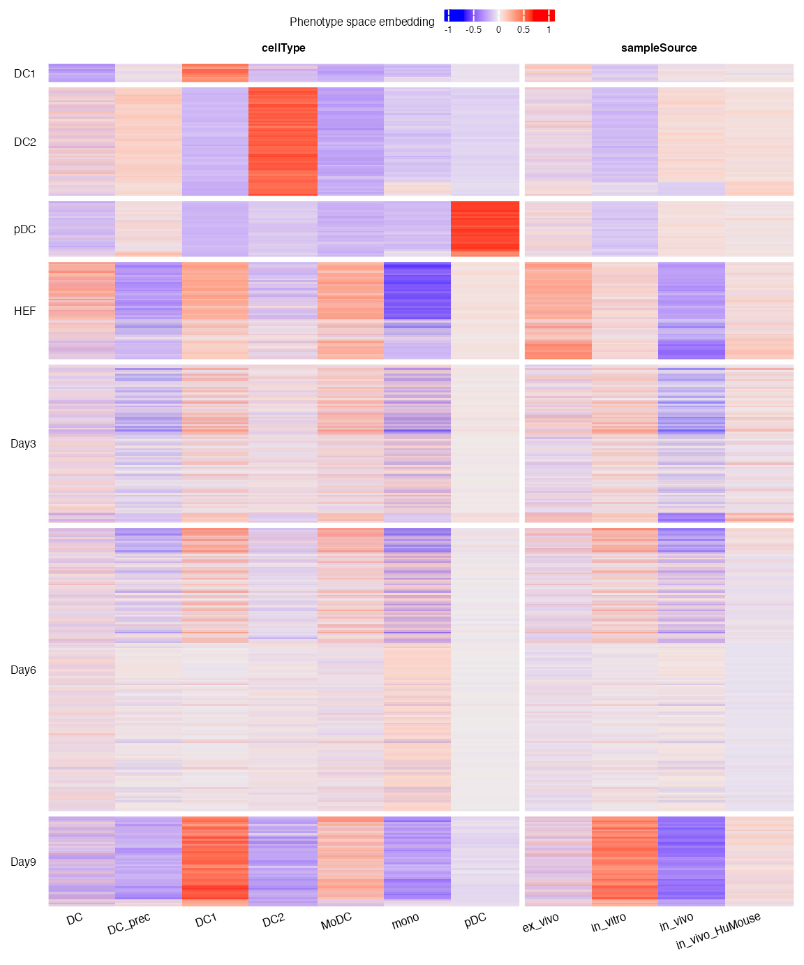

Every column of the heatmap corresponds to a phenotype defined in the bulk reference. Every horizontal line of the heatmap represents a query cell. The query cells are grouped according to their cell types:

Control cell types: DC1 (type 1 conventional DC), DC2 (type 2 conventional DC) and pDC (plasmacytoid DC). These cell types are in vivo DC subtypes;
HEF: the starting point of DC reprogramming;
Day3, Day6, Day9: HEFs after 3, 6 and 9 days of reprogramming.

We can see that the control cell types were predicted to have strong DC1, DC2 and pDC identities. In terms of sample source, they are more in vivo like than in vitro. HEFs have an ambiguous identity since they were not defined in the reference. However, after 9 days of reprogramming, the HEFs were clearly more DC1-like, with strong in vitro identity.

Visualise transitional cell states in phenotype space

The essence of Φ-Space is that we view cell type prediction as dimension reduction. How is it dimension reduction? Look at the heatmap: each cell was represented by the gene expression level of thousands of genes, and now they are represented by 11 dimensions, each measuring their likelihood of belonging to a certain phenotype defined in the reference.

As any other dimension reduction objects, we can use cells’ phenotype space embedding for downstream analyses. One of such analyses is phenotype space PCA, which allows us to visualize both bulk samples and single cells in the same space. The idea is that we first compute a PCA using the phenotype space embeddings of the reference samples, and then project query cells to this PC space via loadings.

queryLabs <- query$mainTypes
queryLabs[queryLabs %in% c("Day9_SP", "Day9_DP")] <- "Day9"
refLabs <- colData(reference)[,"Cell Type"]
YrefHat_norm <- reducedDim(reference, "PhiSpace")
pc_re <- getPC(YrefHat_norm, ncomp = 3)
refEmbedding <- pc_re$scores %>% as.data.frame() %>% mutate(source = reference$`Sample Source`)
# Project query cells via loadings
queryEmbedding <- scale(
    PhiScores_norm, 
    center = T, 
    scale = F
  ) %*% 
  pc_re$loadings %>%
  as.data.frame()

plot_ly(
    x = ~comp1,
    y = ~comp2,
    z = ~comp3,
) %>%
  add_markers(
    data = refEmbedding,
    colors = DC_cols,
    color = refLabs,
    symbol = ~source,
     marker = list(
      size = 5
    )
  ) %>%
  add_markers(
    data = queryEmbedding,
    color = queryLabs, 
    marker = list(
      symbol = ~"x",
      size = 3
    )
  )

Using plotly, we have rendered the PCA results an interactive plot. It is very interesting to observe that, after 9 days of reprogramming, the induced DCs (red crosses) are closer to in vitro rather than in vivo DC1.

PhiSpace parameter tunning

There are two key parameters to select for running PhiSpace annotation:

ncomp: number of PLS (or PCA) components to use for annotation;
nfeat: number of features (eg genes, proteins) to use to predict each phenotype (eg cell type, sample source).

PhiSpace uses a regression model to learn phenotypes, such as cell types, continuously. The parameter ncomp controls the model complexity: setting ncomp too large (small) may cause over-(under-)fitting. nfeat controls how many features PhiSpace uses to make prediction.

PhiSpace provides functions for fully data-driven feature selection based on cross-validation (CV). However, this approach becomes times consuming when the reference sample size becomes large (a common caveat of all CV-based parameter tuning). However, in the current case study where the reference is a bulk atlas, we can still afford to compute CV.

Data-driven parameter tuning (time consuming)

Next we use PhiSpace::tunePhiSpace to do a 5-fold CV grid search. The function will first plot a loss function plot for ncomp and then for nfeat. We will see that ncomp=30 already leads to a very small loss and choosing larger ncomp doesn’t help further reducing loss. Moreover, nfeat = 297 seems to minimise the loss and increasing nfeat will actually increase the loss fucntion.

if(F){ # If you want to run it, change F to T
  tuneRes <- tunePhiSpace(
    reference, assayName = "rank", phenotypes = phenotypes, 
    tune_ncomp = TRUE, tune_nfeat = TRUE, ncomp = c(1,50), nfeatLimits = c(10, 5000),
    Ncores = 4, Kfolds = 5, seed = 5202056
  )
}

After running CV tunning, tuneRes$selectedFeat will return the selected features.

Rule-of-thumb for parameter tunning

As we mentioned, a serious drawback of CV parameter tuning is its high computational cost. Fortunately PhiSpace is quite robust against the value of ncomp and a good rule-of-thumb is to set ncomp to be the number of biologically interesting groups in the data (ie total number of cell types). In the DC case, setting ncomp = 11 will lead to a model that is good enough already. To select nfeat, we can try this simplified approach:

if(!file.exists(paste0(dat_dir, "output/tuneRes.rds"))){
  tuneRes <- tunePhiSpace(
    reference, assayName = "rank", phenotypes = phenotypes, 
    tune_ncomp = F, tune_nfeat = F, ncomp = 11
  )
  qsave(tuneRes, paste0(dat_dir, "output/tuneRes.rds"))
} else {
  tuneRes <- qread(paste0(dat_dir, "output/tuneRes.rds"))
}

In this case, no CV tuning actually happened. Instead, we were telling PhiSpace to stick to ncomp=11 and do not tune nfeat. What is interesting is tuneRes$impScores, which gives the importance score for each gene when used to predict different phenotypes:

head(tuneRes$impScores)

##                 pDC          mono           DC1           DC2       DC_prec
## F2R    5.051386e-04  2.965319e-04 -0.0005824430 -0.0011207552 -4.280220e-04
## OAZ1   7.861188e-06  4.474383e-06 -0.0001510309  0.0001240407  2.849520e-05
## RPS16  2.117688e-04 -1.503983e-04 -0.0001914275  0.0010778257 -5.906239e-04
## RACK1  3.373127e-05 -2.957098e-05 -0.0001195094  0.0002551319 -4.215025e-05
## ORC6  -7.013646e-04 -5.715517e-04  0.0002952676  0.0038080308 -4.329163e-04
## PDCD7 -1.651123e-04 -4.491403e-04 -0.0006121114  0.0024755905 -1.175561e-04
##                  DC          MoDC       in_vivo      in_vitro       ex_vivo
## F2R    8.656067e-04  4.639430e-04 -7.467888e-05 -2.379497e-03  3.550273e-04
## OAZ1  -1.743889e-06 -1.209670e-05 -1.035714e-04  7.210649e-05  2.649781e-05
## RPS16 -1.775075e-04 -1.796372e-04  3.790844e-04 -1.913091e-04 -3.680781e-05
## RACK1 -4.243059e-05 -5.520199e-05  4.011961e-05 -5.205925e-06 -1.232075e-05
## ORC6  -1.853449e-03 -5.440165e-04 -2.888258e-03  1.928230e-03  7.256920e-04
## PDCD7 -7.067049e-04 -4.249654e-04 -1.199273e-03  2.969786e-04  4.904283e-04
##       in_vivo_HuMouse
## F2R      2.099148e-03
## OAZ1     4.967071e-06
## RPS16   -1.509675e-04
## RACK1   -2.259294e-05
## ORC6     2.343365e-04
## PDCD7    4.118664e-04

Then we order the importance of features, in descending order, for each phenotype. Then we can choose the top nfeat features for each cell type.

nfeat <- 300
selRes <- selectFeat(tuneRes$impScores)
head(selRes$orderedFeatMat)

##      pDC     mono      DC1       DC2     DC_prec  DC        MoDC     in_vivo  
## [1,] "KRT5"  "FCGR3A"  "CADM1"   "CYYR1" "OLR1"   "ALDH1A1" "CCL13"  "UQCRH"  
## [2,] "TCL1A" "SLC11A1" "CLEC9A"  "DBN1"  "GLDN"   "FCGR3A"  "CLDN1"  "LYRM2"  
## [3,] "PTCRA" "MS4A4A"  "ENPP1"   "PID1"  "ADAM33" "MS4A4A"  "MMP12"  "EIF1AY" 
## [4,] "MAP1A" "ALDH1A1" "PMP22"   "IL1R1" "RIMS3"  "CCL8"    "SUCNR1" "RPL26"  
## [5,] "LAMP5" "SLAMF1"  "DBN1"    "CD1E"  "FPR3"   "CLC"     "C1QA"   "HSPB11" 
## [6,] "SHD"   "NPL"     "TACSTD2" "PLPP3" "CAMP"   "IDO2"    "CCL8"   "ATP5F1E"
##      in_vitro ex_vivo in_vivo_HuMouse
## [1,] "CCL13"  "C1QB"  "CDKN3"        
## [2,] "CLDN1"  "CLDN1" "AURKB"        
## [3,] "CD1B"   "TFPI"  "CTSG"         
## [4,] "CD1A"   "MMP12" "CKAP2L"       
## [5,] "SUCNR1" "ALPK2" "CDC45"        
## [6,] "MMP12"  "CD1A"  "BUB1"

length(unique(as.character(selRes$orderedFeatMat[1:nfeat,])))

## [1] 1782

For example, we can see that selecting the top 300 features for each cell type, we end up having 1782 genes selected (due to overlapping genes), which should be enough for accurate prediction. In practice, we can adjust the nfeat value till the resulting total number of feature selected reaches a target number (eg the ‘magic number’ 2000 which is used as default number of genes in Seurat).

Jiadong Mao

2025-05-27