Stereo-seq: lineage commitment of AML cells
Jiadong Mao
2025-12-02
StereoSeq.RmdHighlights
Annotation using multiple references;
Annotation of spatial bins (without cell segmentation);
Identify cell states of a large number of cancer clones.
Introduction
In this case study, we will apply PhiSpace to identify clone-specific cell states in an acute myeloid leukaemia (AML) mouse model. The results show that genetically identical AML clones developed different cell states, suggesting that they might commited to different lineages (e.g. lymphocytes vs granulocytes).
- Query: Stereo-seq data from a mouse spleen containing AML cells (Holze et al., 2024).
- Reference: 4 scRNA-seq datasets from healthy and cancerous mouse
spleen, bone marrow and neutrophils
- Spleen: healthy mosue spleen (Zhang et al., 2023);
- BM: healthy mouse bone marrow atlas (Harris et al., 2021);
- CITE: healthy mouse spleen CITE-seq (RNA+surface protein, we only used the RNA part) (Gayoso et al., 2021);
- Neutrophil: single-neutrophil RNA-seq from various types of mosue tissues (healthy and cancerous cell states) (Ng et al., 2024).
In addition, we also make use of a ‘bridge’ dataset as an intermediate between the four reference datasets and the Stereo-seq query:
- Bridge: scRNA-seq from same mouse spleen as the Stereo-seq data (Fennell et al., 2021).
For this case study, utility functions and processed data can all be found in this folder.
# Name of the game
suppressPackageStartupMessages(library(PhiSpace))
suppressPackageStartupMessages(library(vizOmics))
# Tidyverse packages
suppressPackageStartupMessages(library(ggplot2))
## Warning: package 'ggplot2' was built under R version 4.5.2
suppressPackageStartupMessages(library(dplyr))
suppressPackageStartupMessages(library(magrittr))
suppressPackageStartupMessages(library(ggpubr))
suppressPackageStartupMessages(library(tidyr))
# Other utils
suppressPackageStartupMessages(library(qs)) # Fast read and write of large R objects

dat_dir <- "~/Dropbox/Research_projects/PhiSpace/VignetteData/StereoSeq/" # replace this by your own directory

source(paste0(dat_dir, "StereoSeq_utils.R"))
Following Holze et al. (2024), we binned the tissue domain into so-called ‘bin50’ size, resulting in transcript bins with side lengths ~25μm. These bins are larger than typical single cells and hence each bin may contain more than one cell. These bins will be our cell-like objects.
Note on cell segmentation. For subcellular spatial RNA-seq, reliable cell segmentation is not always possible. This is because reliable cell segmentation relies on cell staining such as DAPI and advanced imaging machine learning algorithms (can be time-consuming). And the quality of cell segmentation varies from tissue to tissue, with some tissues such as spleen intrisically difficult to segment due to its complex morphological structures and croweded, overlapping immune cells. If additional cell staining is not included in experimental design (i.e. you unfortunately did pay for it), then cell segmentation cannot be very accurate. In this Stereo-seq case, cell segmentation was not possible due to a phenomenon called ‘swapping’ or ‘bleeding’, i.e. transcripts bleeding among neighbouring measurement units causing contamination. This phenomenon is actually fairly common (no data is perfect!).
queryPath <- paste0(dat_dir, "data/mouse4_bin50_bc_sce.qs")
if(F){ # The data has already been normalised, but if you want to try again, change F to T
  query <- qread(queryPath)
  query <- RankTransf(query, "counts") # Rank transform
  query <- logTransf(query, targetAssay = "log1p", use_log1p = TRUE)
  qsave(query, queryPath)
} else {
  query <- qread(queryPath)
}
Visualise total RNA counts. delete bins with too few transcripts.
VizSpatial(query, ptSize = 1, colBy = "total_counts", fsize = 12)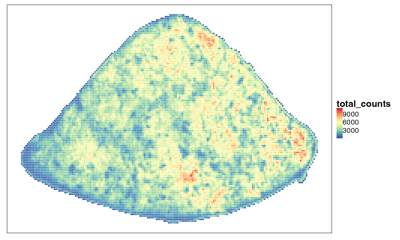
Barcode-seq analysis: defining meta-clones
Decipher evolution of cancer
This Stereo-seq data we analyse here is special since it’s one of the first spatial RNA-seq data with cancer clone lineage tracing information (Holze et al., 2024).
A cancer clone refers to descendants from the same ancestor cell which share identical genome (i.e. same DNA) (Nowell, 1976). Thanks to increasingly cheaper DNA sequencing, we now know that a tumour is usually a patchwork of cancer clones, some more populous and hence more ‘successful’ than others. It is now a consensus that cancer is an evolutionary process, where many different clones compete with each other and the fittest of them survive (Vendramin et al., 2021). Intriguingly enough, this evolutionary process cannot be fully explained by genetics. For example, we now know that some cancer clones are more successful in terms of therapeutic resistance not because they have a more advantageous gene mutations (e.g. a mutation making it easier for them to proliferate), but because of some non-genetic mechanisms (Marine et al., 2020).
The need to understand non-genetic mechanisms underpinning some key cancer evolutionary events, such as therapeutic resistance, motivated the development of SPLINTR (single-cell profiling and lineage tracing), a barcoding technology allowing us to sequencing cancer cells while retaining their clonal identities (Fennell et al., 2022). That is, via SPLINTR we can know which cancer cells belong to the same clone and what are their transcriptional profiles. It is a powerful tool for exploring non-genetic mechanisms since we can see how genetically identical clones develop different transcriptional programs, and hence exhibiting different cell states. Ultimately we might decipher how cancer cells (they are really cunning!) utilise diverse transcriptional programs to evade host immune response and acquire resistance to cancer therapies.
Bibliographic note: the evolutionary theory of cancer hasn’t really been a research focus until recent years after we have access to powerful and more affordable DNA sequencing. But the theoretical framework was discussed as early as 1976 by Peter Nowell in his seminal paper The Clonal Evolution of Tumor Cell Populations. Though people knew very little about cancer genomics back then, the framework of Nowell was suprisingly ahead of his time.
Visualise AML clones
Before plunging into the gene expression space, let’s first look at what SPLINTR tells us about how the AML clones are distributed in the mouse spleen. The input we use here is a so-called barcode-seq file, which is a table telling us which clones are detected and what are their spatial coordinates. Since cells in the same clone have the same SPLINTR barcode, detecting whereabouts of clones is equivalent to detecting whereabouts of barcodes.
# Load barcode-seq
bcRaw <- read.table(
  paste0(dat_dir, "data/mouse4_bin50_bc_counts.tsv"), sep = "\t", header = T, row.names = 1
)
# Match spatial coordinates with sce object
bcRaw$bin_y <- -bcRaw$bin_y
bcRaw$y_center <- -bcRaw$y_center
isin_data <- (bcRaw$isin_adata == "True")
# Simplify barcode names
bcRaw$barcode <- gsub("GFP_", "", bcRaw$barcode)
# Bins that do not contain barcodes
noBarIdx <- setdiff(query$cell_id, bcRaw$cell_id[bcRaw$isin_adata == "True"])
# Show part of barcode-seq
head(bcRaw)
## barcode count_binned bin_x bin_y cell_id x_center y_center isin_adata
## 0 Barcode_32756 13 90 -123 90_123 13645 -17865 False
## 1 Barcode_25 11 -128 -194 -128_194 2745 -21415 False
## 2 Barcode_131914 10 -104 -83 -104_83 3945 -15865 False
## 3 Barcode_131914 9 -124 -207 -124_207 2945 -22065 False
## 4 Barcode_131914 9 208 -22 208_22 19545 -12815 False
## 5 Barcode_2613 8 -35 -103 -35_103 7395 -16865 FalseThere were 370 clones/barcodes detected but most of them were very scarce.
## [1] 370
bcTab[1:30]##
## Barcode_25 Barcode_2613 Barcode_131914 Barcode_25027 Barcode_6595
## 5428 3073 2922 1376 1183
## Barcode_19949 Barcode_5687 Barcode_25727 Barcode_42724 Barcode_32756
## 814 723 707 490 470
## Barcode_12424 Barcode_1190 Barcode_8 Barcode_1794 Barcode_120950
## 435 328 320 280 238
## Barcode_87074 Barcode_10626 Barcode_3036 Barcode_70639 Barcode_1209
## 189 174 122 115 114
## Barcode_49666 Barcode_108275 Barcode_150642 Barcode_146599 Barcode_69630
## 114 103 103 99 90
## Barcode_50878 Barcode_43 Barcode_28543 Barcode_6537 Barcode_5925
## 85 82 73 70 67
bcTab[341:370]##
## Barcode_62985 Barcode_67039 Barcode_68225 Barcode_6850 Barcode_6957
## 1 1 1 1 1
## Barcode_70428 Barcode_70487 Barcode_7114 Barcode_71766 Barcode_7262
## 1 1 1 1 1
## Barcode_73834 Barcode_74003 Barcode_76770 Barcode_79993 Barcode_80014
## 1 1 1 1 1
## Barcode_8051 Barcode_82825 Barcode_82916 Barcode_8369 Barcode_84496
## 1 1 1 1 1
## Barcode_87623 Barcode_88641 Barcode_88652 Barcode_88815 Barcode_8942
## 1 1 1 1 1
## Barcode_91999 Barcode_922 Barcode_93569 Barcode_95213 Barcode_9983
## 1 1 1 1 1We visualise the spatial distributions of some of the dominating clones. This helps us see if a clone tends to concentrate within a spatial region, and if different clones tend to concentrate in different regions. In solid tumours (e.g. lung tumours) clones are normally clustered together spatially but we are dealing with liquid tumour here (leukaemia) so the spatial clonal patterns are not well understood.
We first define some useful quantities for plotting.
# Which coordinates to use
xCoordName <- "x_center"
yCoordName <- "y_center"
# X and Y limits
xylimits <- bcRaw[isin_data, c(xCoordName, yCoordName)] %>% apply(2, quantile, probs = c(0,1))
## Convex hull defining spleen region
ch <- colData(query)[, c("x", "y")] %>% as.matrix()
ch <- ch[chull(ch),]
sortedBC <- table(bcRaw$barcode) %>% sort(decreasing = T)
We first plot the density of all clones using two-dimensional kernel
density estimation (KDE). This tells us if AML cells tend to occupy
certain spatial niches or that they are spreading evenly. (Need to
install ks package for kernel smoothing.)
xx_eval <- colData(query)[query$barcode != "nan", c("x", "y")]
xx <- colData(query)[query$barcode != "nan", c("x", "y")]
# install.packages("ks")
suppressWarnings(kde_res <- tempDenPlot(xx, xx_eval, xylimits, ch, F, psize = 1, "", spleenOnly = F))
estValues <- kde_res$kde_res$estimate
estRange <- range(estValues)
kde_res$p + scale_colour_gradientn(colours = PhiSpace:::MATLAB_cols, limits = estRange) 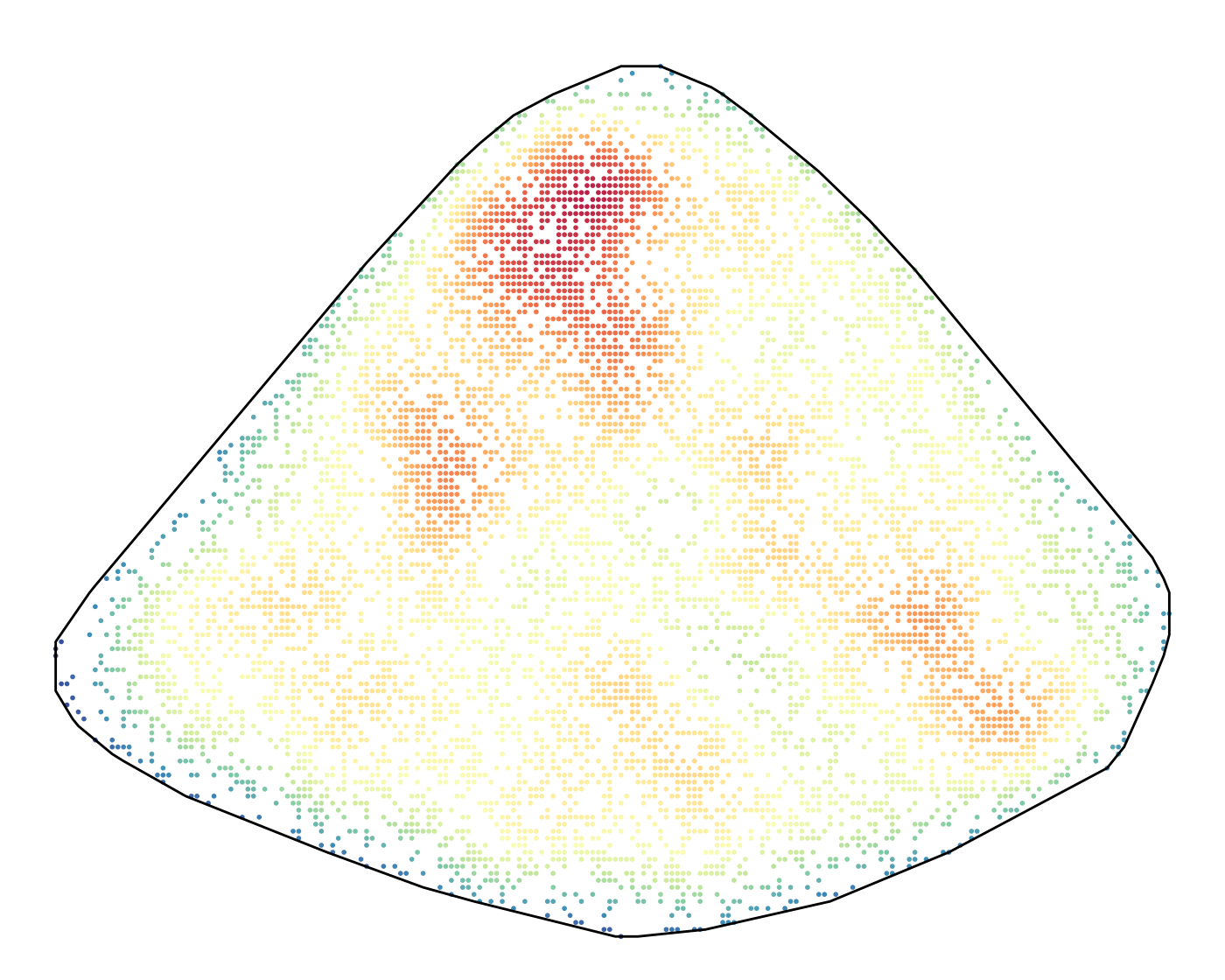
Overall AML cells seemed to clustered in space. We then do KDE for the top 16 clones.
sortedBC <- table(bcRaw$barcode) %>% sort(decreasing = T)
xx_eval <- bcRaw[, c(xCoordName, yCoordName)] %>% `colnames<-`(c("x", "y"))
kdePath <- paste0(dat_dir, "output/cloneKDEres.qs")
if(!file.exists(kdePath)){
  out <- lapply(
    1:16,
    function(x){
      # Which clone
      bcName <- names(sortedBC)[x]
      # Data for density est
      xx <- bcRaw[bcRaw$barcode == bcName, c(xCoordName, yCoordName)]
      suppressWarnings(kde_res <- tempDenPlot(xx, xx_eval, xylimits, ch, F, psize = 0.3, bcName, spleenOnly = T))
      return(kde_res)
    }
  )
  qsave(out, kdePath)
} else {
  out <- qread(kdePath)
}
estValues <- lapply(out, function(x) x$kde_res$estimate) %>% unlist
estRange <- range(estValues)
outPlots <- lapply(
  out,
  function(x){
    p <- x$p
    suppressMessages(
      p <- p + scale_colour_gradientn(colours = PhiSpace:::MATLAB_cols, limits = estRange)
    )
  }
)
ggarrange(plotlist = outPlots, nrow = 4, ncol = 4, legend = "none")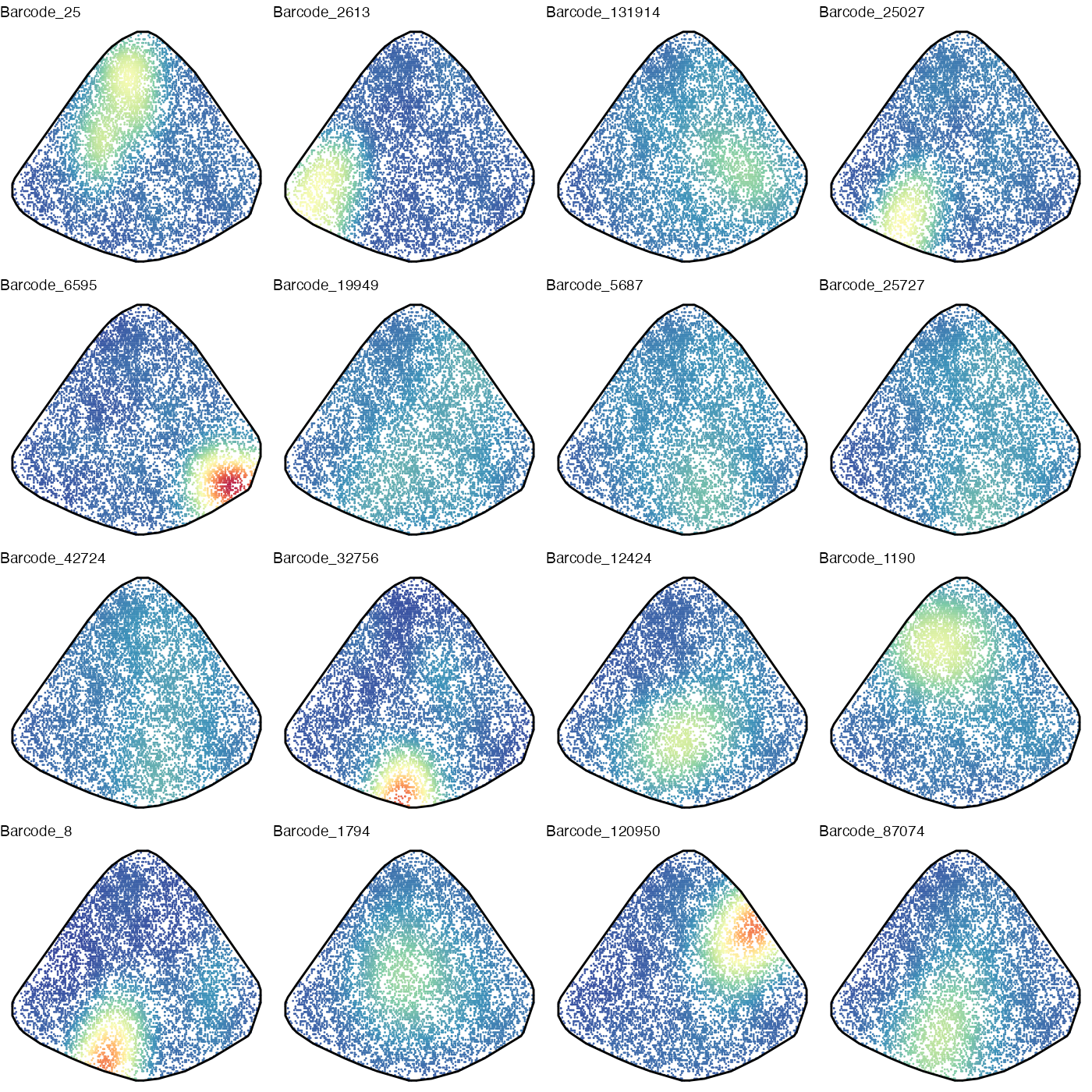
These individual KDE plots revealed some spatial patterns of individual clones. The most populous clone with Barcode_25, for example, tended to occupy the top left corner. Some clones, such as Barcode_19949, tended to spread out more evenly.
Define meta-clones
How do we summarise the spatial patterns of all these clones? Instead of viewing them one by one, we aggregate the high abundance clones into meta-clones.
We first filter out low abundance barcodes. The idea is that, most barcodes have very low abundance (e.g. detected in only one bin) and it’s not very interesting analysing them here since they do not tell us much about how AML clones tend to be distributed in space. However this doesn’t mean that the low-abundance clones are not biologically important. Some rare clones may not seem very successful when cancer is expanding but they might be able to develop resistance to, say, chemotherapy, so they might take over after chemo. All we are saying here is that the low-abundance clones can be left out in the currently analysis of spatial patterns, which really rely on higher-abundance clones to provide more statistical power.
sortedBC_filt <- sortedBC[sortedBC >= 50]
length(sortedBC_filt)
## [1] 35
bcFilt <- bcRaw %>% filter(barcode %in% names(sortedBC_filt)) %>%
  mutate(barcode = as.factor(barcode))
We only kept 35 clones with more than 50 cells each. Next we cluster the Stereo-seq bins according to their composition of clones. That is, two bins will belong to the same cluster, which we call a meta-clone, if they have similar composition of individual clones. However, due to the relatively small bin size (~25μm), each bin contained only a few barcode. Hence we do some spatial smoothing as follows.
For a given Stereo-seq bin, we count the barcodes present in the
surrounding bins whose distances to that given bin is no larger than
xyRange. We selected xyRange <- 50 and
noted that the specific value of xyRange doesn’t tend to
change the clustering results much.
xyRange <- 500
binIDs <- unique(bcFilt$cell_id)
barAssay <- sapply(
  1:length(binIDs),
  function(x){
    binID <- binIDs[x]
    coords <- bcFilt %>% filter(cell_id == binID)
    coords <- coords[1, c("x_center", "y_center")]
    xcond <- (abs(bcFilt$x_center - coords[1,1]) < xyRange)
    ycond <- (abs(bcFilt$y_center - coords[1,2]) < xyRange)
    idx <- xcond & ycond
    table(bcFilt[idx,"barcode"])
  }
) %>% t() %>% `rownames<-`(binIDs)
Next we cluster the bins with smoothed out clonal composition using k-means. We try different choices of number of clusters.
Note on k-means: the default setting of
kmeans in R is actually inappropriate for many
applications. First, kmeans uses random initialisation of
cluster centroid, so each run of it may give you slightly different
clustering results. It’s almost always a good idea to set
nstart to be some large number such as 50, so that the
function will run k-means for multiple times and selected the best one
(with tighter clusters) as final output. Second thing is that the
default maximal number of iterations controlled by iter.max
is set to be too small (only 10) by default. The clustering often cannot
converge with such as small number of iterations. So it needs to be set
larger by hand. My personal guess is that R inherits its early
implementation of k-means, when the number of iterations had to be set
small due to limited computing resource.
plot_dat <- unique(bcFilt[,c("cell_id", xCoordName, yCoordName)]) %>% as.data.frame()
clustPath <- paste0(dat_dir,"output/barcode-seq_clustering.qs")
if(!file.exists(clustPath)){
  set.seed(523423)
  outClusts <- lapply(
    2:10,
    function(kclust){
      clust_res <- kmeans(barAssay, centers = kclust, iter.max = 100, nstart = 50)
      return(clust_res)
    }
  )
  qsave(outClusts, clustPath)
} else {
  outClusts <- qread(clustPath)
}
Next we visualise the clusters, or meta-clones. The idea is to select
a number of meta-clones based on this visualisation. Now a trick we use
in PhiSpace is to align the clusters across different
clustering results, so that two clusters similar to each other will
receive the same label. This cluster alignment is done by
PhiSpace::align_clusters. This is actually a very useful
functionality as clusters in clustering algorithms are arbitrarily
named. So even the same cluster in two cluster results might be labelled
differently (e.g. labelled 1 in one run of k-means, labelled 2 in
another). This will make their visualisation harder to compare since
even the same cluster will receive two colours across two results.
Technical note: we align the clusters using the
Hungarian algorithm implemented by clue::solve_LSAP.
Similar clusters across different cluster results will be labelled using
the same number.
clust_list <- lapply(
  outClusts,
  function(x) factor(x$cluster, levels = sort(unique(x$cluster)))
)
# Align clusters across different results
outPlots <- vector("list", length(clust_list))
for(x in length(clust_list):1){
  clust <- clust_list[[x]]
  if(x < length(clust_list)){
    clust_old <-  clust_list[[x+1]]
    clust <- align_clusters(clust, clust_old) %>% as.factor()
    clust_list[[x]] <- factor(clust, levels = as.character(sort(as.numeric(levels(clust)))))
  }
  plot_dat <- plot_dat %>%  mutate(clusters = clust_list[[x]])
  outPlots[[x]] <- tempClustPlot(plot_dat, T, pSize = 0.3)
}
suppressWarnings(ggarrange(plotlist = outPlots, nrow = 3, ncol = 3, legend = "none"))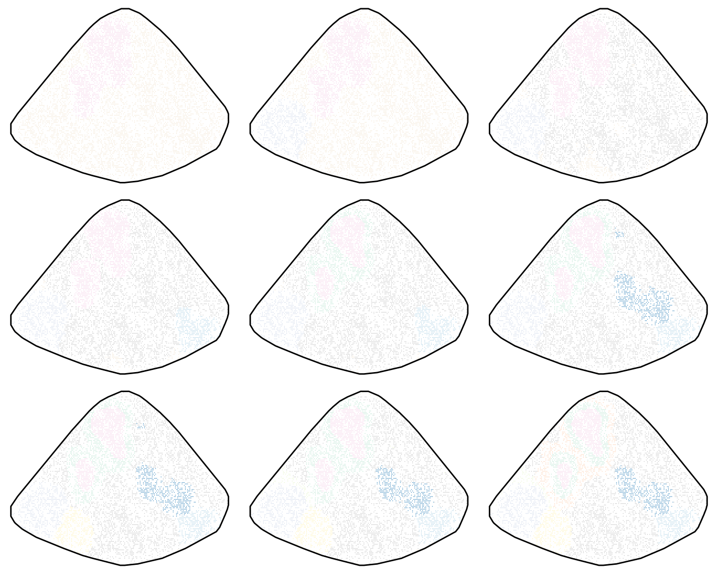
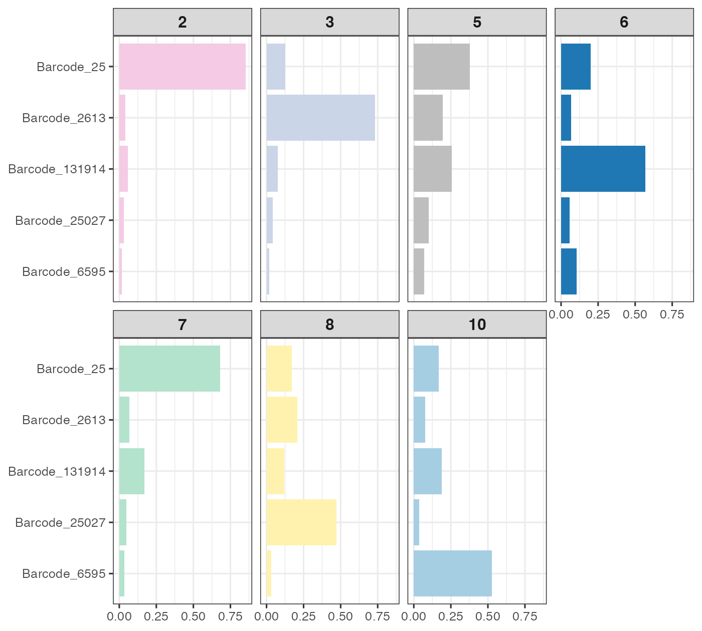
Some meta-clones, such as the pink one, appeared very early, even when there were only two clusters. This means that these clones are more significant in some sense. To interpret the clusters, we look at clone composition of each cluster.
binIDs <- unique(bcFilt$cell_id)
barAssayRaw <- sapply(
  1:length(binIDs),
  function(x){
    binID <- binIDs[x]
    idx <- (bcFilt$cell_id == binID)
    table(bcFilt[idx,"barcode"])
  }
) %>% t() %>% `rownames<-`(binIDs)
clustIdx <- 7
clust <- clust_list[[clustIdx]]
barSelected <- names(sortedBC)[1:5]
plot_dat_wide <- barAssayRaw[,barSelected] %>% as.data.frame() %>%
  mutate(clust = clust) %>% group_by(clust) %>%
  summarise(across(starts_with("Barcode"), sum))
plot_prop <- plot_dat_wide %>% select(!clust) %>% as.matrix()
plot_prop <- (plot_prop/rowSums(plot_prop)) %>% as.data.frame() %>%
  mutate(clust = plot_dat_wide$clust) %>%
  pivot_longer(!clust, values_to = "count", names_to = "barcode") %>%
  mutate(barcode = factor(barcode, levels = rev(barSelected)))
plot_prop <- plot_prop %>% filter(clust != "9")
plot_prop %>% ggplot(aes(count, barcode)) +
  geom_bar(aes(fill = clust), stat = "identity") + theme_bw(base_size = 12) +
  scale_fill_manual(values = clust_cols) + facet_wrap(~ clust, nrow = 2) +
  theme(
    legend.position = "none", axis.title = element_blank(),
    strip.text.x = element_text(size = 12, face = "bold")
  )
tempClustPlot(plot_dat %>% mutate(clusters = clust_list[[clustIdx]]), T, pSize = 1.5) +
  theme_void(base_size = 12) + theme(legend.position = "top")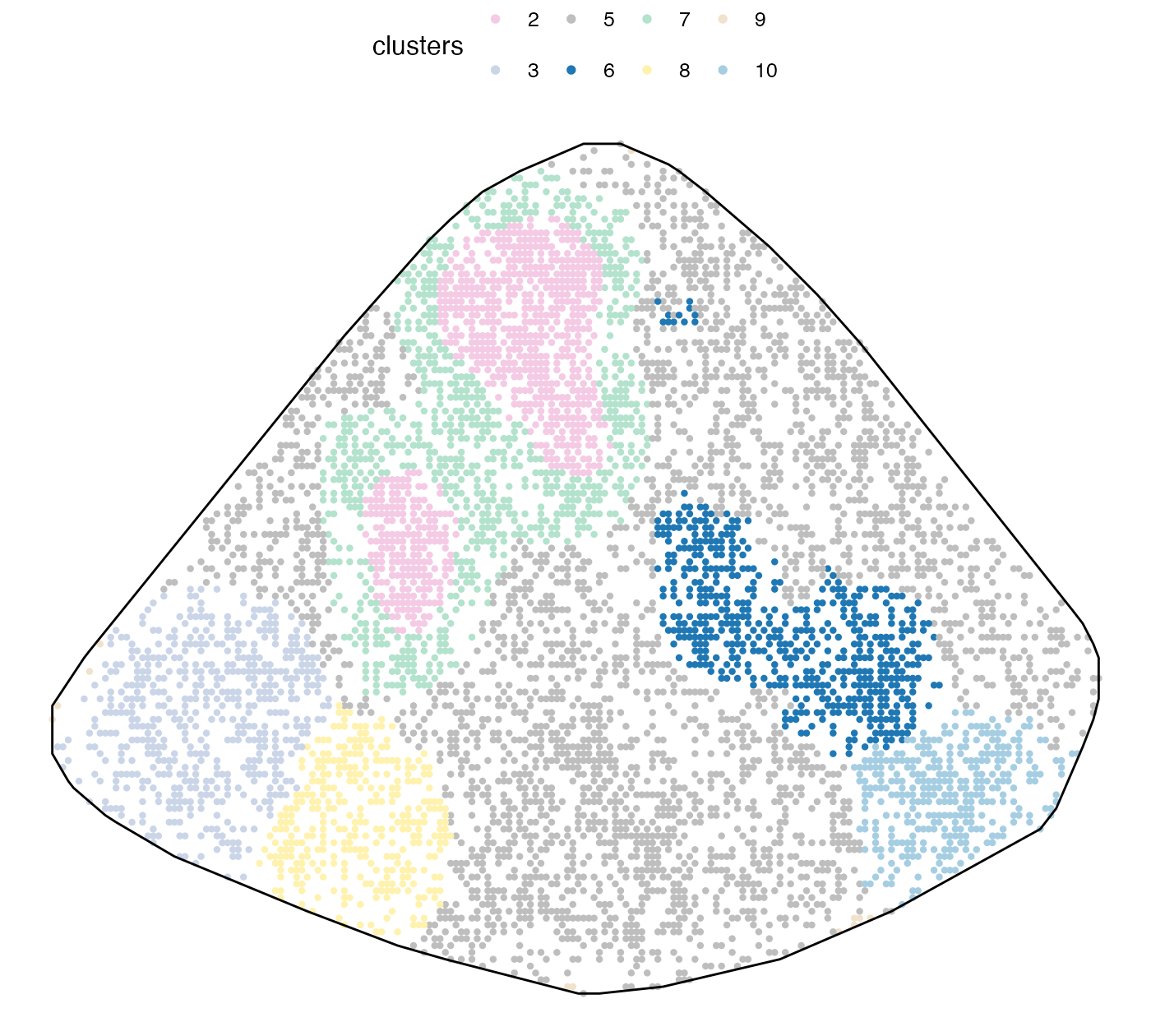
We picked number of meta-clones equal to 8 since most meta-clones contained 1 dominant barcode, except for clone 5, which contained a bit of everything and did really show an interesting spatial pattern. Note that meta-clone 9 was excluded since most of its cells were located outside the spleen region, depicted by the black solid line. This is a technical artefact we discussed above.
PhiSpace analyses
After knowing how clones tended to be located in the spleen sample, we now look at their cell states. As mentioned above, the experiment was designed so that all clones have the same DNA, so they are ideal for identifying non-genetic differences between AML clones.
Since the same mouse spleen was subjected to both Stereo-seq and scRNA-seq, we use the matched scRNA-seq as a ‘bridge’ to enhance the annotation of spatial bins. The idea is that we first use the four scRNA-seq references to annotate the bridge scRNA-seq, and then use the annotated bridge scRNA-seq to annotate Stereo-seq. The reasoning for this bridging approach is that, technically, the references and the bridge datasets are more similar and, biologically, the bridge and the query Stereo-seq datasets are more similar. It turns out that the PhiSpace annotation makes more sense using the bridging approach compared to directly annotating the query using the references.
Annotation of the bridge dataset is tedious and requires larger memory to run (see our source code on GitHub for details). So here we only show how to use the annotated bridge scRNA-seq to annotate the query Stereo-seq from the same mouse spleen.
PhiResPath <- paste0(dat_dir, "output/PhiRes.qs")
if(!file.exists(PhiResPath)){
  querySC <- qread(paste0(dat_dir, "data/mouse4_scRNAseq_sce.qs"))
  pathPhiSc <- paste0(dat_dir, "output/Mouse4_scRNA-seq_PhiSc_list.rds")
  impScPath <- paste0(dat_dir, "output/ImpScores_for_Mouse4_scRNA-seq.rds")
  scPhiSc_list <- readRDS(pathPhiSc)
  reducedDim(querySC, "PhiSpace") <- do.call("cbind", scPhiSc_list)
  newNames <- c(
    "RBC", "CD8 T", "Plasma", "Mature B", "cDC",
    "NK", "Neutro", "CD4 T", "Cr2 B", "HSPC",
    "Trans B", "Mono", "T", "Pre-B cycl", "Endo",
    "Cd7+ NK", "Macro", "pDC", "Baso", "Pre-B",
    "Mono", "Naive B", "Granulo", "Macro", "Imm B",
    "HPC", "Late pro-B", "Imm NK", "ProEryThBla", "T",
    "ErythBla", "T3", "MAT 3", "MAT 2", "IMM 1",
    "MAT 4", "MAT 1", "IMM 2", "T1", "T2",
    "PreNeu", "MAT 5", "MZ B", "Trans B", "Mat B",
    "CD122+ B", "Ifit3+CD4 T", "CD4 T", "pDC", "CD8 T",
    "B1 B", "NKT", "Ifit3+ B", "NK", "GD T",
    "ICOS+ Tregs", "Tregs", "Ly6+ mono", "Neutro", "Cycl B/T",
    "cDC2", "Ly6- mono", "RedPulp macro", "RBC", "Mig DC",
    "Ifit3+CD8 T", "cDC1", "Act CD4 T", "Plasma", "MZ/Marco+ macro"
  )
  newNames <- paste0(
    newNames,
    rep(c("(Spleen)", "(BM)", "(Neutro)", "(CITE)"), sapply(scPhiSc_list, ncol))
  )
  colnames(reducedDim(querySC, "PhiSpace")) <- newNames
  querySC <- logTransf(querySC, targetAssay = "log1p", use_log1p = T)
  PhiRes <- PhiSpaceR_1ref(
    querySC, query, response = reducedDim(querySC, "PhiSpace"),
    PhiSpaceAssay = "log1p", nfeat = 500, regMethod = "PLS", scale = FALSE
  )
  qsave(PhiRes, PhiResPath)
} else {
  PhiRes <- qread(PhiResPath)
}
reducedDim(query, "PhiSpace") <- normPhiScores(PhiRes$PhiSpaceScore)[colnames(query),]
Next we visualise some cell types. First we observed a strong neutrophil identity, represented by Neutro(Spleen), Granulo(BM) and T2(Neutro) cell types in different references (neutrophil in spleen, granulocytes (including neutrophil) in bone marrow and a cancer-associated neutrophil labelled T2). And the strong neutrophil identity coincides with the biggest clone (see above). What is also interesting is the distribution of erythrocytes. Several references confirmed that there is a strong erythrocyte identity towards the right boundary of spleen (e.g. erythroblast visualised below). Moreover, we observed that the macrophage identity delineates ring-like structures, which potentially correspond to the right-like marginal zones in spleen. Naive B cell, on the other hand, delineates what are potentially the white pulps.
VizSpatial(query, ptSize = 1, reducedDim = "Neutro(Spleen)", censor = T, fsize = 12)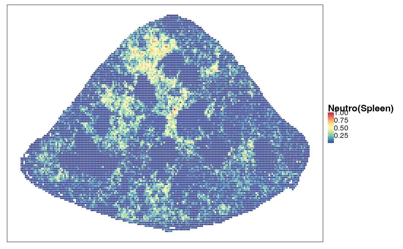
VizSpatial(query, ptSize = 1, reducedDim = "Granulo(BM)", censor = T, fsize = 12)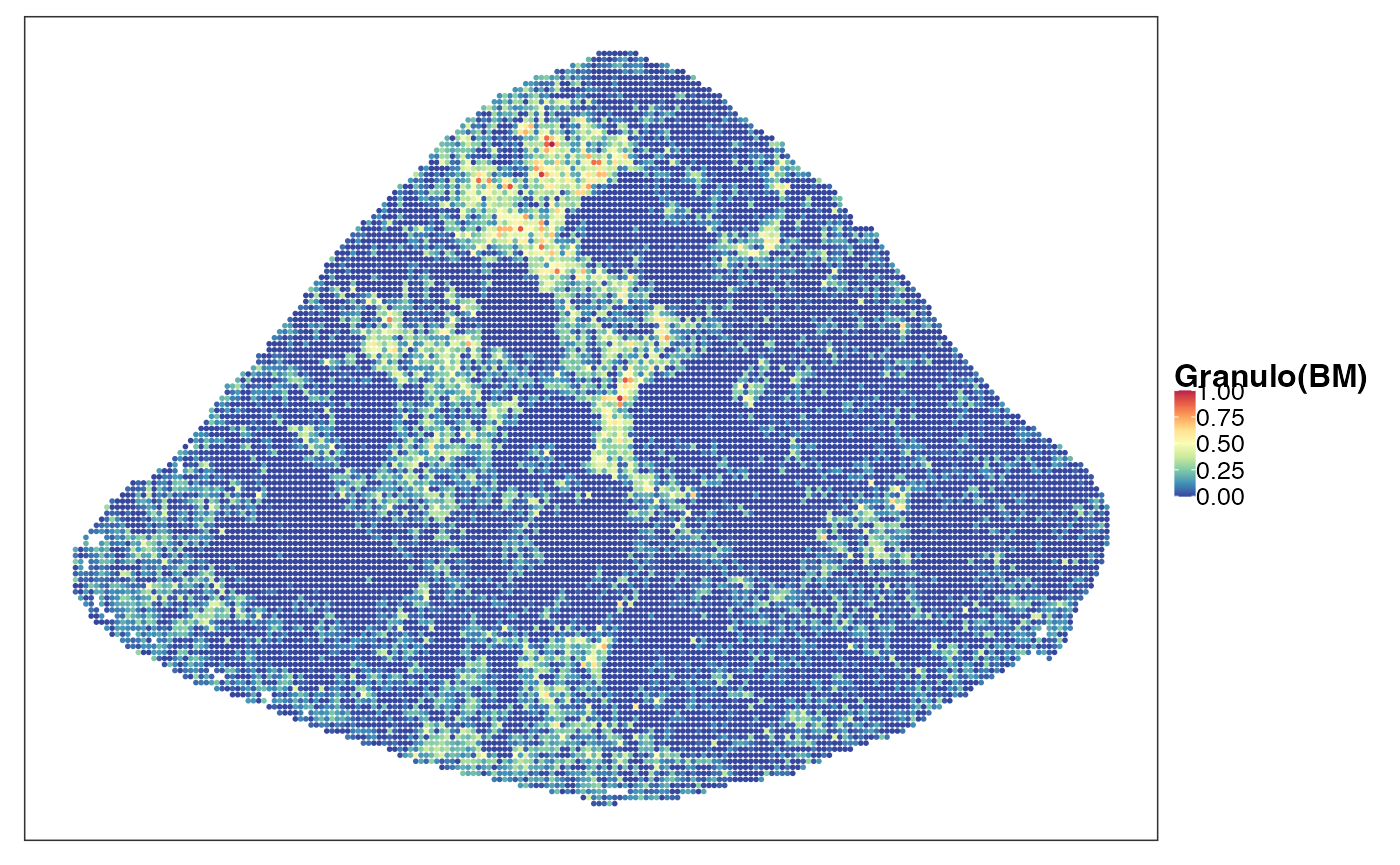
VizSpatial(query, ptSize = 1, reducedDim = "T2(Neutro)", censor = T, fsize = 12)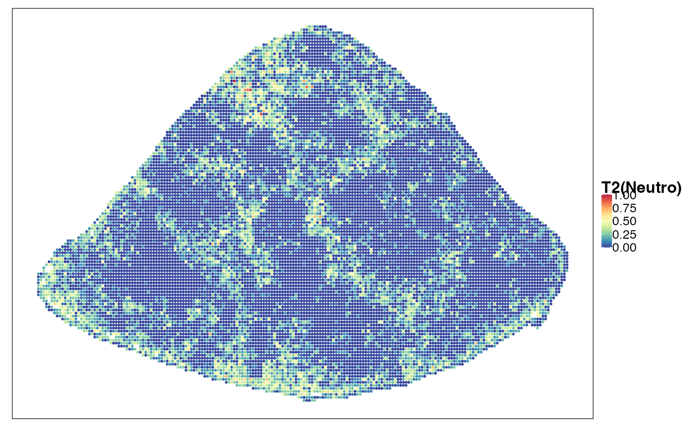
VizSpatial(query, ptSize = 1, reducedDim = "ErythBla(BM)", censor = T, fsize = 12)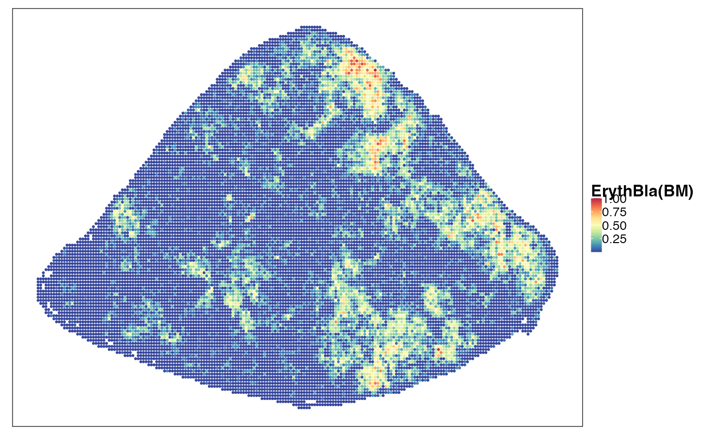
VizSpatial(query, ptSize = 1, reducedDim = "Macro(Spleen)", censor = T, fsize = 12)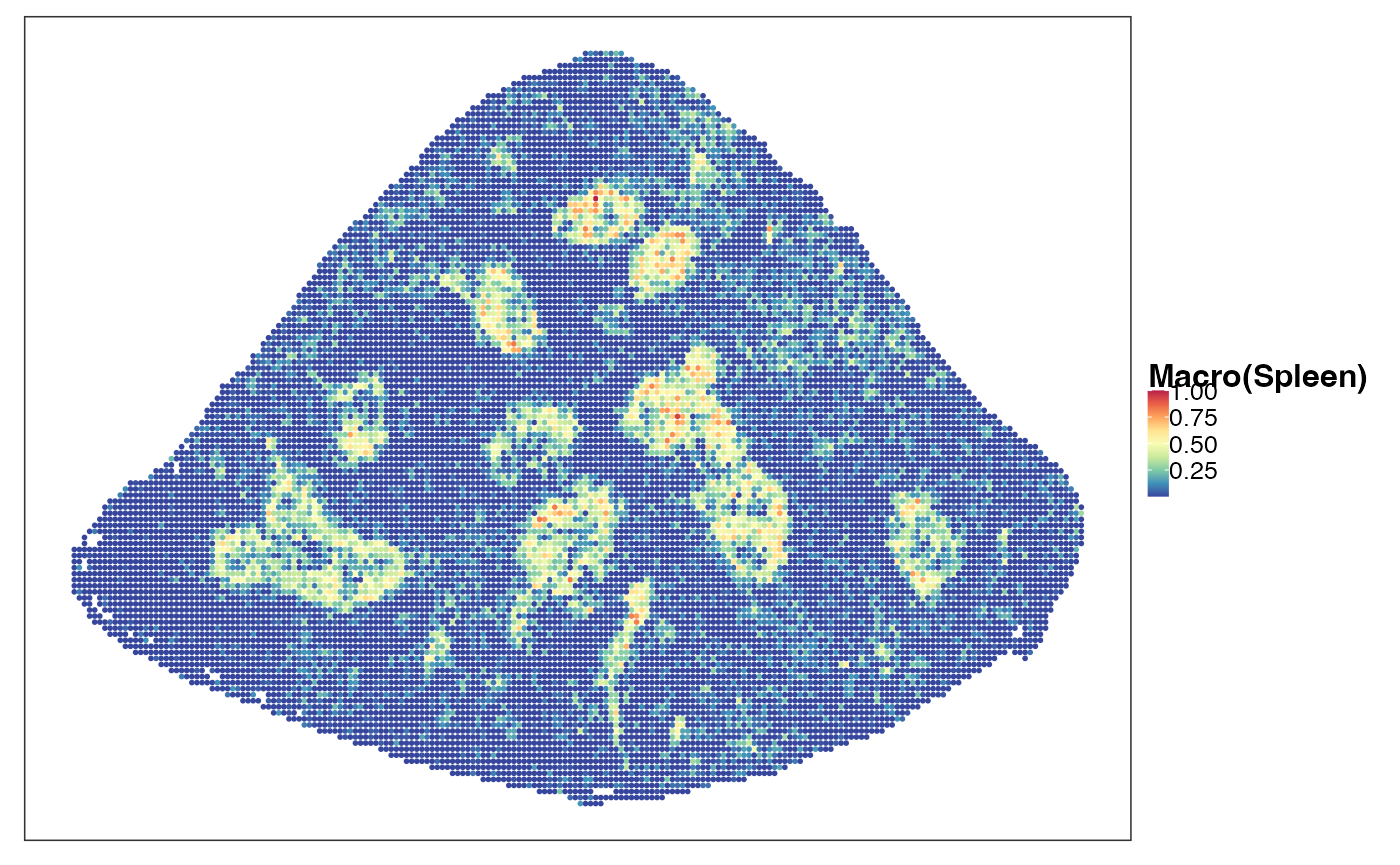
VizSpatial(query, ptSize = 1, reducedDim = "Naive B(BM)", censor = T, fsize = 12)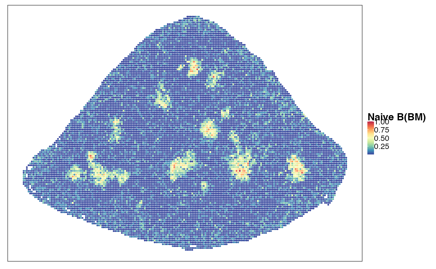
Next we cluster the PhiSpace cell type scores to identify spatial niches. Note how niche 4 (red) seems to represent the marginal zone and niche 7 (blue) seems to represent the white pulps. Niche 8 (green) represents the location of the largest AML clone (see above).
tempClustCols <- c(
  "1" = "#FF7F00", "2" = "#377EB8", "3" = "#F781BF", "4" = "#984EA3",
  "5" = "#A65628", "6" = "#4DAF4A", "7" = "#FFFF33", "8" = "#E41A1C"
)
pathPhiClustRes <- paste0(dat_dir, "output/PhiClustRes.qs")
if(!file.exists(pathPhiClustRes)){
  PhiPCRes <- getPC(reducedDim(query, "PhiSpace"), ncomp = ncol(reducedDim(query, "PhiSpace")) - 1)
  PhiPCRes$accuProps
  plot(1-PhiPCRes$accuProps)
  mat2clust <- PhiPCRes$scores[,1:30]
  names(tempClustCols) <- 1:8
  set.seed(94863)
  clust_res <- kmeans(mat2clust, centers = 8, iter.max = 200L, nstart = 50)
  qsave(clust_res, pathPhiClustRes)
} else {
  clust_res <- qread(pathPhiClustRes)
}
query$PhiClust <- as.character(clust_res$cluster)
VizSpatial(query, colBy = "PhiClust", ptSize = 1, legend.symb.size = 2) +
  scale_colour_manual(values = tempClustCols) +
  theme(legend.title = element_text(face = "bold"), legend.key.spacing = unit(0, "pt"))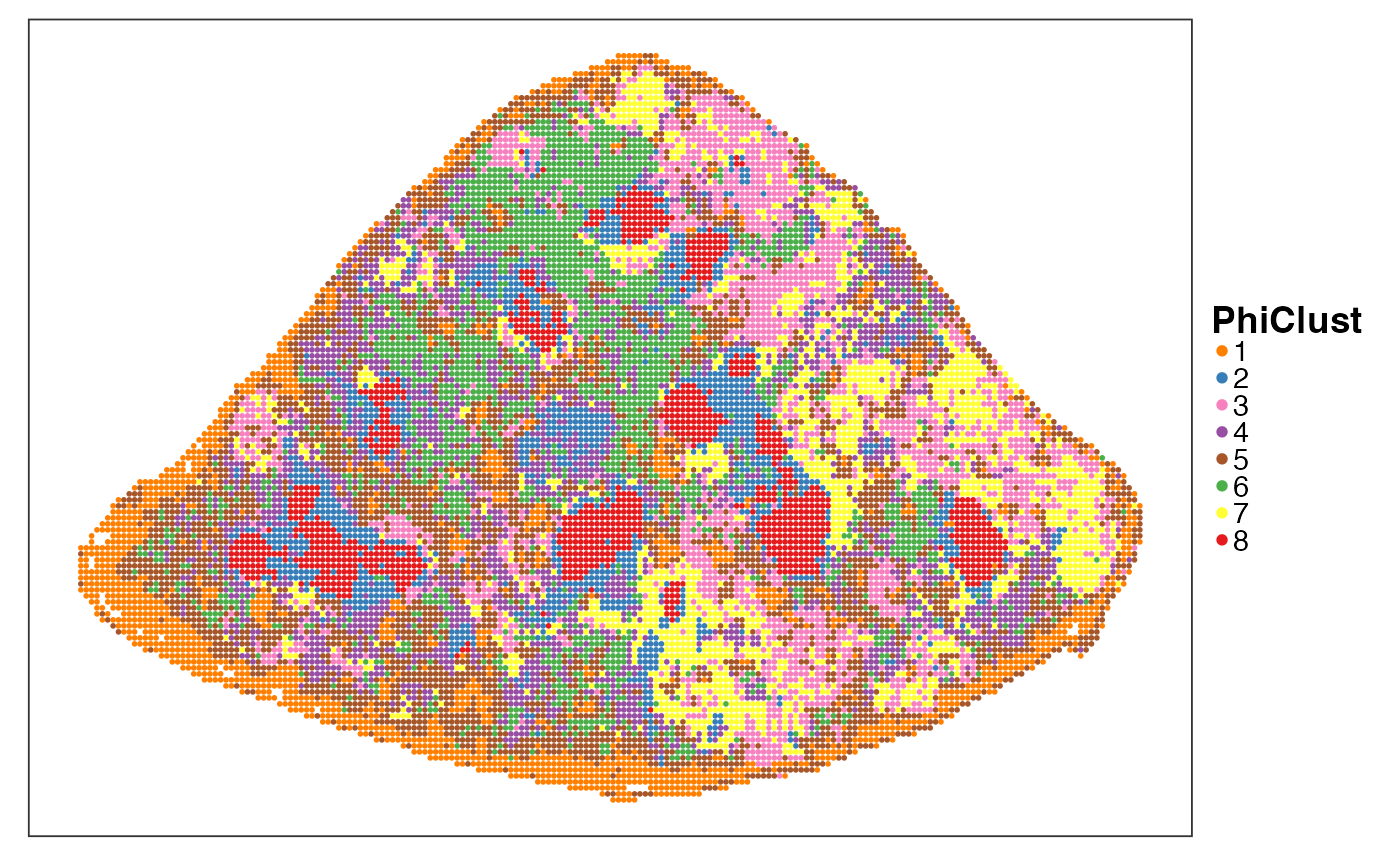
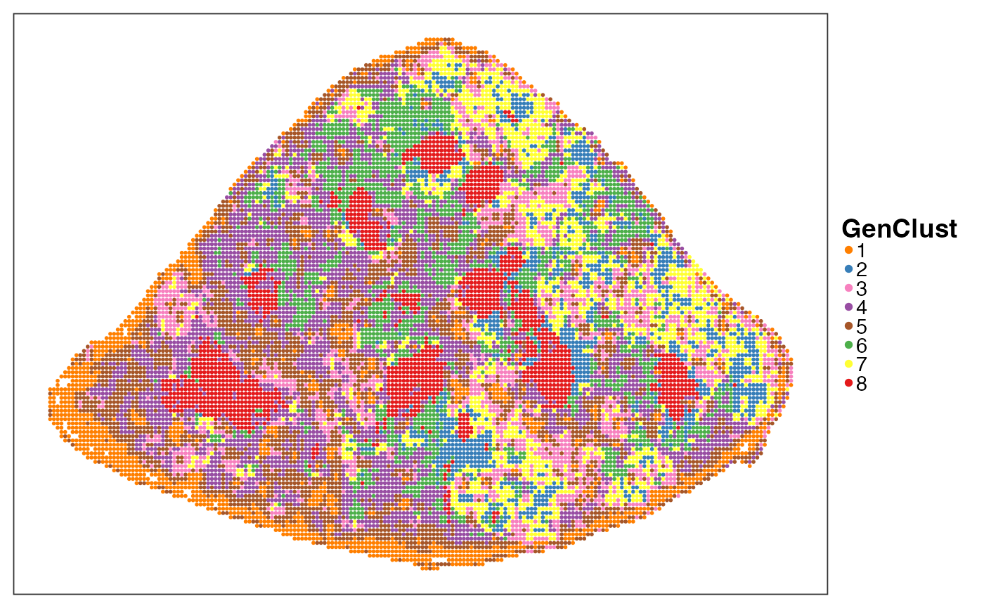
In contrast, we can cluster the Stereo-seq bins according to their gene expression to identify the same number of spatial niches as above. The features highlighted by PhiSpace niches, i.e. marginal zone, white pulp and largest clone, were lost.
pathGexClustRes <- paste0(dat_dir, "output/GexClustRes.qs")
if(!file.exists(pathGexClustRes)){
  mat2clust <- getPC(t(assay(query, "log1p")), ncomp = 30)$scores
  set.seed(94858)
  clust_res <- kmeans(mat2clust, centers = 8, iter.max = 200L, nstart = 50)
  qsave(clust_res, pathGexClustRes)
} else {
  clust_res <- qread(pathGexClustRes)
}
query$GenClust <- align_clusters(as.character(clust_res$cluster), query$PhiClust)
VizSpatial(query, colBy = "GenClust", ptSize = 1) +
  scale_colour_manual(values = tempClustCols) +
  guides(colour = guide_legend(override.aes = list(size = 2))) +
  theme(
    legend.title = element_text(face = "bold"),
    legend.position = "right", legend.key.spacing = unit(0, "pt")
  )
We use DWD (see CosMx case study) to compare barcoded and non-barcoded bins. Here barcoded bins refer to Stereo-seq bins where at least one barcode was detected.
library(kerndwd)
barcodeVec <- as.character(query$barcode)
barcodeVec[barcodeVec != "nan"] <- 1
barcodeVec[barcodeVec == "nan"] <- -1
barcodeVec <- as.numeric(barcodeVec)
X_cent <- reducedDim(query, "PhiSpace") %>% as.matrix()
X_cent <- scale(X_cent, center = T, scale = F)
lambda = 10^(seq(-2, -5, length.out=50))
kern = vanilladot()
cv_res = cv.kerndwd(X_cent, barcodeVec, kern, qval=1, lambda=lambda, eps=1e-5, maxit=1e5)
da_res = kerndwd(X_cent, barcodeVec, kern, qval=1, lambda=cv_res$lambda.min, eps=1e-5, maxit=1e5)
dwdLoad <- da_res$alpha[-1,,drop=F] %>% `dimnames<-`(list(colnames(X_cent),"comp1")) # worked out by looking at predict.dwd
dwdScore <- predict.kerndwd(da_res, kern, X_cent, X_cent, "link") %>% `colnames<-`("comp1")
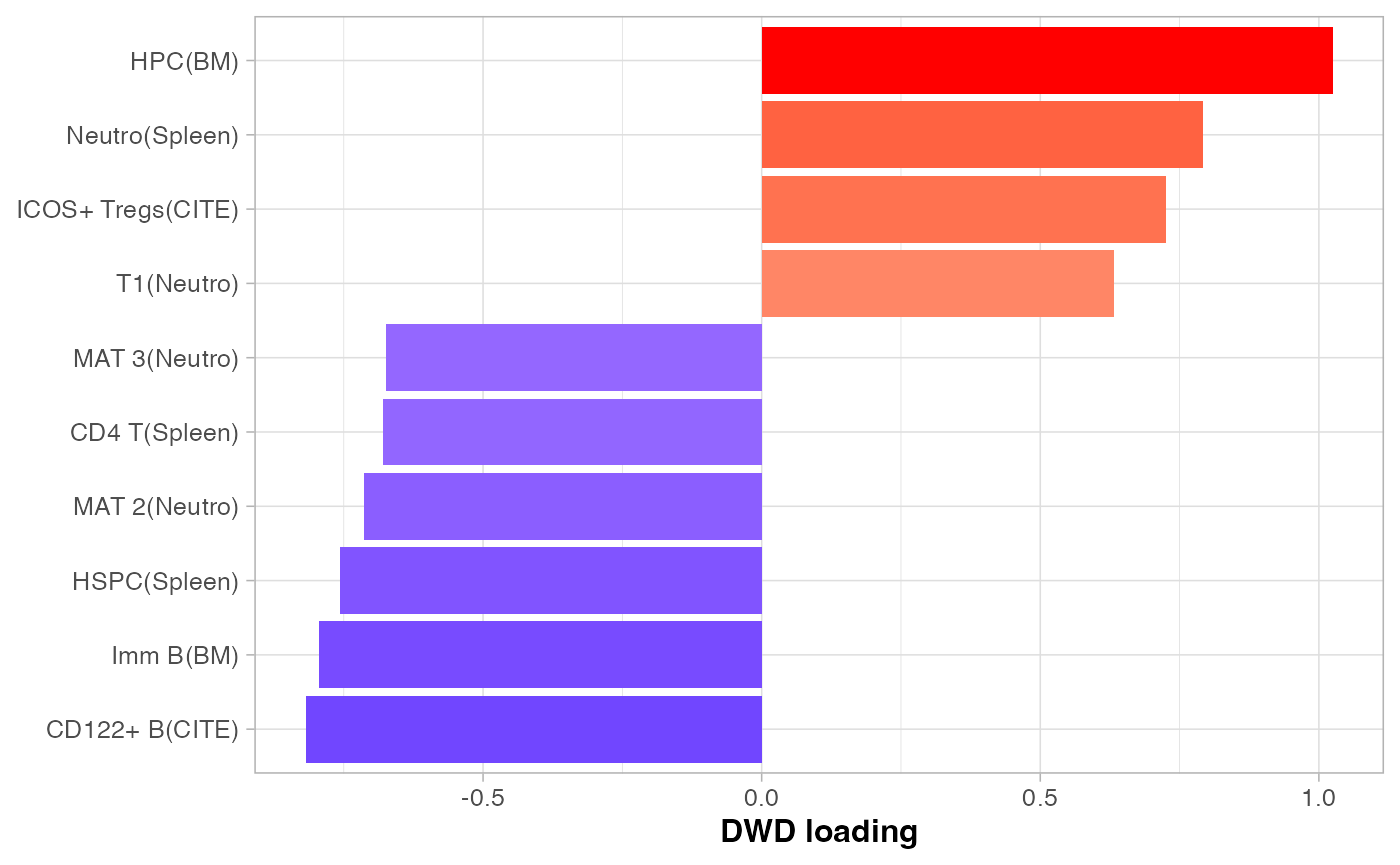
dwd_res <- list(scores = dwdScore %>% as.data.frame(), loadings = dwdLoad %>% as.data.frame())It seems that barcoded and non-barcoded bins were somewhat separable. And the cell type signals explaining their separation were also plotted. This low level of separation (compared to those seen in Visium and CosMx case studies) is expected, since we are analysing a liquid cancer at its late metastasis stage in the current case study. This means that the cancer cells permeated the poor mouse’s spleen so the barcoded and non-barcoded bins might not be easily distinguishable.
barcodedOrNo <- barcodeVec
barcodedOrNo[barcodeVec==1] <- "Barcoded"
barcodedOrNo[barcodeVec==-1] <- "Nonbarcoded"
dwd_res$scores %>% mutate(niche = barcodedOrNo) %>% ggplot() +
  geom_density(aes(comp1, fill = niche), alpha = 0.5) +
  theme_pubr(base_size = 12) + theme(legend.title = element_blank()) + xlab("DWD score")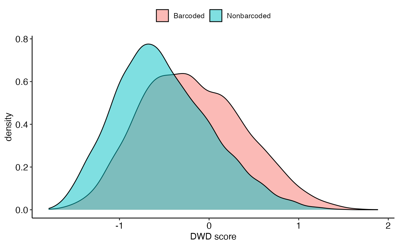
plotLoadings(
  dwd_res$loadings, comp = "comp1", showInt = F,
  nfeat = 10, fsize = 12, xlab = "DWD loading", absVal = T
)
Recall that we defined meta-clones summarising spatial territories of individual clones. We can now look at how these meta-clones differ in terms of their cell states. Note that the neutrophil identity was enriched in meta-clone 2, which is consistent with what we’ve been observing.
clustBar <- clust_list[[clustIdx]] %>% `names<-`(rownames(barAssay)) # containing all barcoded bins in and out spleen
plot_dat <- reducedDim(query, "PhiSpace") %>% as.data.frame()
clustBar <- clustBar[intersect(rownames(plot_dat), names(clustBar))]
clust <- rep("background", nrow(plot_dat))
names(clust) <- rownames(plot_dat)
clust[names(clustBar)] <- as.character(clustBar)
# Select some clusters
selectedClust <- c("2", "3", "5", "6", "7", "8", "10", "background")
clust <- clust[clust %in% selectedClust]
clust <- factor(clust, levels = selectedClust)
plot_dat <- plot_dat[names(clust), ] %>%
    mutate(cluster = clust, x = query[,names(clust)]$x, y = query[,names(clust)]$y)
cTypes <- colnames(reducedDim(query, "PhiSpace"))
suppressWarnings(
  p_boxs <- tempSaveBox(plot_dat, cTypes, width = 7, height = 10, fignrow = 8, figncol = 9, fsize = 5, returnPlot = T, savePlots = F)
)
p_boxs$`Neutro(Spleen)` + theme_bw(base_size = 12) +
  theme(legend.position = "top",axis.text.y = element_text(), legend.title = element_text(face = "bold")) +
  guides(fill = guide_legend(nrow = 1))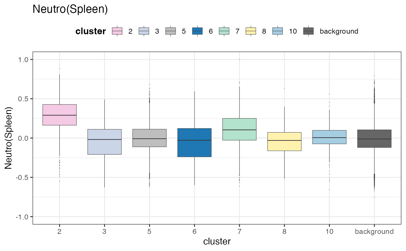
We conduct statistical tests to see which clusters have differentially enriched cell types compared to background (non-barcoded bins). Interestingly, these meta-clones, defined according to their spatial locations, tended to have cell states corresponding to different lineage. However, meta-clones close to each other tended to have similar cell states (in terms on lineage). Overall, we observed three types of cell states:
Neutrophil-like: meta-clones 2 and 7;
Myeloid-like: meta-clones 3 and 8;
Erythrocyte-like: meta-clones 6.
pathSigScores <- paste0(dat_dir, "output/sigScores.qs")
if(!file.exists(pathSigScores)){
  cTypes <- colnames(reducedDim(query, "PhiSpace"))
  pvals <- sapply(
    cTypes,
    function(cType){
      sc_split <- split(reducedDim(query, "PhiSpace")[names(clust),cType], clust)
      bkgrd <- sc_split$background
      sc_split[["background"]] <- NULL
      testRes <- sapply(sc_split, function(x) wilcox.test(x, bkgrd)$p.value)
      return(testRes)
    }
  ) %>% t()
  fc <- sapply(
    cTypes,
    function(cType){
      sc_split <- split(reducedDim(query, "PhiSpace")[names(clust),cType], clust)
      bkgrd <- sc_split$background
      sc_split[["background"]] <- NULL
      foldChange <- sapply(sc_split, function(x) (mean(x) - mean(bkgrd))/sd(bkgrd))
      return(foldChange)
    }
  ) %>% t()
  sigScores <- fc * (-log10(pvals)) # feature significance score
  qsave(sigScores, pathSigScores)
} else {
  sigScores <- qread(pathSigScores)
}
# most enriched
tab <- selectFeat(sigScores, absVal = F)$orderedFeatMat[1:5, !(colnames(sigScores) %in% c("5","9"))]
knitr::kable(tab)| 2 | 3 | 6 | 7 | 8 | 10 |
|---|---|---|---|---|---|
| Neutro(Spleen) | CD8 T(Spleen) | T1(Neutro) | HPC(BM) | HPC(BM) | HPC(BM) |
| Granulo(BM) | Imm NK(BM) | cDC1(CITE) | Neutro(Spleen) | CD8 T(Spleen) | HSPC(Spleen) |
| Neutro(CITE) | T(BM) | MAT 5(Neutro) | Ly6+ mono(CITE) | Ly6+ mono(CITE) | CD8 T(Spleen) |
| HPC(BM) | HPC(BM) | cDC(Spleen) | IMM 1(Neutro) | Pre-B cycl(Spleen) | pDC(Spleen) |
| IMM 1(Neutro) | Pre-B cycl(Spleen) | Mono(BM) | Granulo(BM) | Imm NK(BM) | B1 B(CITE) |